


扫一扫
关注中图网
官方微博


本类五星书更多>
-
>
宇宙、量子和人类心灵

-
>
(精)BBC地球故事系列-星际旅行
-
>
从一到无穷大
-
>
图说相对论(32开平装)
-
>
一本有趣又有料的化学书
-
>
刘薰宇的数学三书:原来数学可以这样学全3册
-
>
光学零件制造工艺学


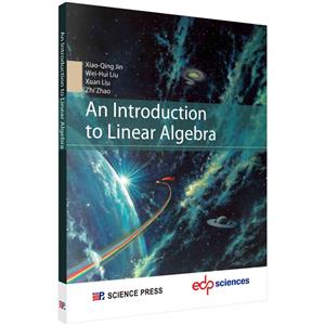
线性代数导引 版权信息
- ISBN:9787030721631
- 条形码:9787030721631 ; 978-7-03-072163-1
- 装帧:一般胶版纸
- 册数:暂无
- 重量:暂无
- 所属分类:>
线性代数导引 内容简介
近年来,随着能源环境问题日益凸显和轻量化设计制造的需求日益迫切,航空航天、轨道交通、节能汽车等高技术领域对原位铝基复合材料的需求潜力巨大,且对其综合性能的要求也越来越高。本书较系统、详细地介绍了原位铝基复合材料的体系设计、材料开发、制备技术、凝固组织、塑变加工及性能。全书共八章,主要内容包括:原位反应体系的设计与开发、电磁法合成原位铝基复合材料、高能超声法合成原位铝基复合材料、声磁耦合法合成原位铝基复合材料、原位铝基复合材料的凝固组织及界面结构、塑变加工对原位铝基复合材料组织的影响、原位铝基复合材料的力学性能、原位铝基复合材料的磨损性能。内容丰富、新颖,具有系统性和前瞻性,反映了作者团队二十余年来在原位铝基复合材料领域的科研成果。
线性代数导引 目录
Contents
Chapter 1 Linear Systems and Matrices 1
1.1 Introduction to Linear Systems and Matrices 1
1.1.1 Linear equations and linear systems 1
1.1.2 Matrices 3
1.1.3 Elementary row operations 4
1.2 Gauss-Jordan Elimination 5
1.2.1 Reduced row-echelon form 5
1.2.2 Gauss-Jordan elimination 6
1.2.3 Homogeneous linear systems 9
1.3 Matrix Operations 11
1.3.1 Operations on matrices 11
1.3.2 Partition of matrices 13
1.3.3 Matrix product by columns and by rows 13
1.3.4 Matrix product of partitioned matrices 14
1.3.5 Matrix form of a linear system 15
1.3.6 Transpose and trace of a matrix 16
1.4 Rules of Matrix Operations and Inverses 18
1.4.1 Basic properties of matrix operations 19
1.4.2 Identity matrix and zero matrix 20
1.4.3 Inverse of a matrix 21
1.4.4 Powers of a matrix 23
1.5 Elementary Matrices and a Method for Finding A.1 24
1.5.1 Elementary matrices and their properties 24
1.5.2 Main theorem of invertibility 26
1.5.3 A method for finding A.1 27
1.6 Further Results on Systems and Invertibility 28
1.6.1 A basic theorem 28
1.6.2 Properties of invertible matrices 29
1.7 Some Special Matrices 31
1.7.1 Diagonal and triangular matrices 32
1.7.2 Symmetric matrix 34
Exercises 35
Chapter 2 Determinants 42
2.1 Determinant Function 42
2.1.1 Permutation, inversion, and elementary product 42
2.1.2 Definition of determinant function 44
2.2 Evaluation of Determinants 44
2.2.1 Elementary theorems 44
2.2.2 A method for evaluating determinants 46
2.3 Properties of Determinants 46
2.3.1 Basic properties 47
2.3.2 Determinant of a matrix product 48
2.3.3 Summary 50
2.4 Cofactor Expansions and Cramer’s Rule 51
2.4.1 Cofactors 51
2.4.2 Cofactor expansions 51
2.4.3 Adjoint of a matrix 53
2.4.4 Cramer’s rule 54
Exercises 55
Chapter 3 Euclidean Vector Spaces 61
3.1 Euclidean n-Space 61
3.1.1 n-vector space 61
3.1.2 Euclidean n-space 62
3.1.3 Norm, distance, angle, and orthogonality 63
3.1.4 Some remarks 65
3.2 Linear Transformations from Rn to Rm 66
3.2.1 Linear transformations from Rn to Rm 66
3.2.2 Some important linear transformations 67
3.2.3 Compositions of linear transformations 69
3.3 Properties of Transformations 70
3.3.1 Linearity conditions 70
3.3.2 Example 71
3.3.3 One-to-one transformations 72
3.3.4 Summary 73
Exercises 74
Chapter 4 General Vector Spaces 79
4.1 Real Vector Spaces 79
4.1.1 Vector space axioms 79
4.1.2 Some properties 81
4.2 Subspaces 81
4.2.1 Definition of subspace 82
4.2.2 Linear combinations 83
4.3 Linear Independence 85
4.3.1 Linear independence and linear dependence 86
4.3.2 Some theorems 87
4.4 Basis and Dimension 88
4.4.1 Basis for vector space 88
4.4.2 Coordinates 89
4.4.3 Dimension 91
4.4.4 Some fundamental theorems 93
4.4.5 Dimension theorem for subspaces 95
4.5 Row Space, Column Space, and Nullspace 97
4.5.1 Definition of row space, column space, and nullspace 97
4.5.2 Relation between solutions of Ax = 0 and Ax=b 98
4.5.3 Bases for three spaces 100
4.5.4 A procedure for finding a basis for span(S) 102
4.6 Rank and Nullity 103
4.6.1 Rank and nullity 104
4.6.2 Rank for matrix operations 106
4.6.3 Consistency theorems 107
4.6.4 Summary 109
Exercises 110
Chapter 5 Inner Product Spaces 115
5.1 Inner Products 115
5.1.1 General inner products 115
5.1.2 Examples 116
5.2 Angle and Orthogonality 119
5.2.1 Angle between two vectors and orthogonality 119
5.2.2 Properties of length, distance, and orthogonality 120
5.2.3 Complement 121
5.3 Orthogonal Bases and Gram-Schmidt Process 122
5.3.1 Orthogonal and orthonormal bases 122
5.3.2 Projection theorem 125
5.3.3 Gram-Schmidt process 128
5.3.4 QR-decomposition 130
5.4 Best Approximation and Least Squares 133
5.4.1 Orthogonal projections viewed as approximations 134
5.4.2 Least squares solutions of linear systems 135
5.4.3 Uniqueness of least squares solutions 136
5.5 Orthogonal Matrices and Change of Basis. 138
5.5.1 Orthogonal matrices 138
5.5.2 Change of basis 140
Exercises 144
Chapter 6 Eigenvalues and Eigenvectors 149
6.1 Eigenvalues and Eigenvectors 149
6.1.1 Introduction to eigenvalues and eigenvectors 149
6.1.2 Two theorems concerned with eigenvalues 150
6.1.3 Bases for eigenspaces 151
6.2 Diagonalization 152
6.2.1 Diagonalization problem 152
6.2.2 Procedure for diagonalization 153
6.2.3 Two theorems concerned with diagonalization 155
6.3 Orthogonal Diagonalization 156
6.4 Jordan Decomposition Theorem 160
Exercises 162
Chapter 7 Linear Transformations 166
7.1 General Linear Transformations 166
7.1.1 Introduction to linear transformations 166
7.1.
展开全部
线性代数导引 节选
Chapter 1 Linear Systems and Matrices “No beginner’s course in mathematics can do without linear algebra,” —Lars Garding “Matrices act They don’t just sit there.” —Gilbert Strang Solving linear systems (a system of linear equations) is the most important problem of linear algebra and possibly of applied mathematics as well. Usually, information in a linear system is often arranged into a rectangular array, called a “matrix”. The matrix is particularly important in developing computer programs to solve linear systems with huge sizes because computers are suitable to manage numerical data in arrays. Moreover, matrices are not only a simple tool for solving linear systems but also mathematical objects in their own right. In fact, matrix theory has a variety of applications in science, engineering, and mathematics. Therefore, we begin our study on linear systems and matrices in the first chapter. 1.1 Introduction to Linear Systems and Matrices Let IR denote the set of real numbers. We now introduce linear equations, linear systems, and matrices. 1.1.1 Linear equations and linear systems We consider where are coefficients,are variables (unknowns), n is a positive integer, and 6 G R is a constant. An equation of this form is called a Zinear equation, in which all variables occur to the first power., the linear equation is called a homogeneous linear equation. A sequence of numbers si, sn is called a solution of the equation if,xn = sn such that The set of all solutions of the equation is called the solution set of the equation. In the book, we always use example(s) to make our points clear. Example We consider the following linear equations: (a) (b) It is easy to see that the solution set of (a) is a line in xy-plane and the solution set of (b) is a plane in xyz-space. We next consider the following m linear equations in n variables: (1-1) where are coefficients,are variables, and bi are constants. A system of linear equations in this form is called a linear system. A sequence of numbers si,is called a solution of the system if,is a solution of each equation in the system. A linear system is said to be consistent if it has at least one solution.Otherwise, a linear system is said to be inconsistent if it has no solution. Example Consider the following linear system The graphs of these equations are lines called li and We have three possible cases of lines l\ and I2 in xy-plane. See Figure 1.1. When l\ and I2 are parallel, there is no solution of the system. When li and I2 intersect at only one point, there is exactly one solution of the system. When l1 and I2 coincide, there are infinitely many solutions of the system. Figure 1.1 1.1.2 Matrices The term matrix was first introduced by a British mathematician James Sylvester in the 19th century. Another British mathematician Arthur Cayley developed basic algebraic operations on matrices in the 1850s. Up to now, matrices have become the language to know. Definition A matrix is a rectangular array of numbers. The numbers in the array are called the entries in the matrix. Remark The size of a matrix is described in terms of the number of rows and columns it contains. Usually, a matrix with m rows and n columns is called an m x n matrix. If A is an m x n matrix, then we denote the entry in row i and column j of A by the symbol (A)ij = a々.Moreover, a matrix with real entries will be called a real matrix and the set of all m x n real matrices will be denoted by the symbol Rmxn. For instance, a matrix A in IRmxn can be written as where G IR for any i and j. When compactness of notation is desired, the preceding matrix can be written as We now introduce some important matrices with special sizes. A row matrix is a general 1 x n matrix a given by The main diagonal of the square matrix A is the set of entries an, (1.2) For linear system (1.1), we can write it briefly as the following matrix form which is called the augmented matrix of (1.1). Remark When we construct an augmented matrix associated with a given linear system, the unknowns must be written in the same order in each equation and the constants must be on the right. 1.1.3 Elementary row operations In order to solve a linear system efficiently, we replace the given system with its augmented matrix and then solve the same system by operating on the rows of the augmented matrix. There are three elementary row operations on matrices defined as follows: (1) Interchange two rows. (2) Multiply a row by a nonzero number. (3) Add a multiple of one row to another row. By using elementary row operations, we can always reduce the augmented matrix of a given system to a simpler augmented matrix from which the solution of the system is evident. See the following example. 1.2 Gauss-Jordan Elimination In this s
书友推荐
- >
名家带你读鲁迅:朝花夕拾

名家带你读鲁迅:朝花夕拾
¥10.5¥21.0 - >
罗庸西南联大授课录
罗庸西南联大授课录
¥13.8¥32.0 - >
月亮与六便士
月亮与六便士
¥13.4¥42.0 - >
我与地坛
我与地坛
¥16.8¥28.0 - >
人文阅读与收藏·良友文学丛书:一天的工作
人文阅读与收藏·良友文学丛书:一天的工作
¥16.0¥45.8 - >
诗经-先民的歌唱
诗经-先民的歌唱
¥15.9¥39.8 - >
有舍有得是人生
有舍有得是人生
¥21.2¥45.0 - >
山海经
山海经
¥20.4¥68.0
本类畅销
-

时间简史-普及版
¥16.3¥38 -
数学的魅力;初等数学概念演绎
¥10.8¥22 -
图说相对论(32开平装)
¥14.7¥46 -
刘薰宇的数学三书:原来数学可以这样学全3册
¥35.4¥118 -
中职对口升学数学复习指导
¥23.1¥30 -
高等数学基础
¥31.5¥45